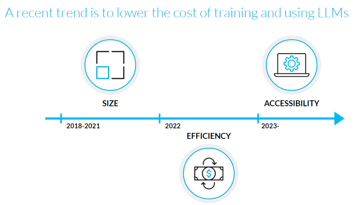
More than a year has passed since the release of ChatGPT, which led hundreds of millions of people to not only talk about AI, but actively use it on a daily basis. The wide adoption of ChatGPT and other large language models (LLMs) among individuals made companies of all sizes and across all sectors of industry wonder how they could benefit from this upward-trending technology. One of the main challenges with turning LLMs into business value is the high cost of the expensive hardware required to run the models. Fortunately, recent developments in the field have allowed companies to significantly lower these expenses.
This article will be a summary of the most recent trends around LLMs, focusing on LLM democratization – making generative AI easily accessible to everyone. The two main topics we will dive into are quantized inference and parameter-efficient fine-tuning. Apart from explaining these concepts and stressing their importance, we will share our experience from their practical use in commercial LLM projects which we have recently delivered to our clients.
If you want to know more about the history of large language models, their different “flavors” and example applications, feel free to check out our report or watch our deeptalk.
LLMs for everyone – the recent trend of AI democratization
ChatGPT is an example (not the first of its kind but undoubtedly the most famous one) of a large language model. LLMs are machine learning models based on deep neural networks, capable of generating text by autoregressively predicting the next word (or the next token, to be more precise). Their applications range from answering questions based on provided documents or knowledge bases (so-called retrieval-augmented generation, or RAG for short), to text summarization, content creation, coding assistants and more.
The most powerful models like those from OpenAI (ChatGPT, GPT-4), Google (Gemini Ultra) and several open-source alternatives (Falcon, Llama 2 or Mixtral, to name a few) are astonishingly performant, even superior to humans in many tasks. Their power can be unleashed thanks to the fact that they are large, i.e. they consist of dozens or hundreds of billions of so-called parameters – numbers that describe how to convert the input data into an output text.
Between 2018 and 2021, based on the visibly improving capabilities of increasingly larger models, the direction set in the field by the world’s biggest research labs was to push the model size to the extreme. However, with the large size comes many challenges, with the high cost of hardware (GPUs with enough memory) required not only for training the model but even serving it for inference being one of the main limitations and factors making business decision makers hesitant to build products or try to improve existing processes with the help of LLMs.
Fortunately, around early 2022, LLM researchers started to understand that for the LLMs to be practically applicable, scaling the models further up was not the way to go. Instead, they turned their attention to training so-called compute-optimal models, which paved the way for all the much smaller (with “only” a few billion parameters), yet still powerful, language models developed both by big tech companies and the open-source community in 2023.
In parallel to the models, motivated by the need to reduce costs and broaden access to the technology, new algorithms and ideas around quantized inference and parameter-efficient fine-tuning have been developed. We will delve into the details in the following sections.
LLM quantization – reducing the memory required for inference
The larger the model, the more GPU memory it needs to load its parameters into. Typically, billions of parameters require gigabytes of RAM. But how many exactly? To answer this question, we will first describe the various ways in which numbers (and hence the model parameters as well) can be represented.
Numeric data types
Two common floating-point formats used in deep learning applications include the single-precision floating-point format (known as FP32) and the half-precision floating-point format (FP16). FP32 utilizes 32 bits for representing a floating-point number, distributing 1 bit for the sign, 8 bits for the exponent, and 23 bits for the significand (see Figure 2), whereas FP16 allocates 16 bits, dividing them into 1 bit for the sign, 5 bits for the exponent, and 10 bits for the significand. It is worth mentioning one more data type, designed specifically with deep neural networks in mind – bfloat16 (brain floating point). Numbers in this format are also represented with 16 bits, but composed differently: 1 sign bit, 8 exponent bits (same as FP32), and 7 bits for the significand. In this way, despite bfloat16’s lower numerical precision, its dynamic range is equivalent to that of FP32.
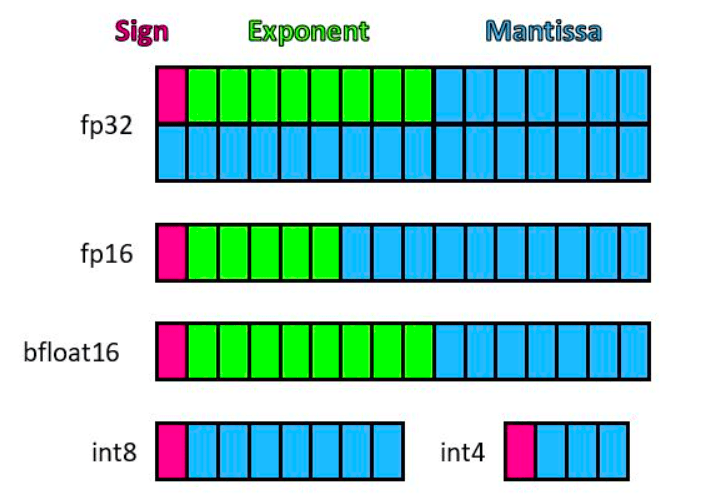 Figure 2. Illustration of various numeric data types, source: https://www.microsoft.com/en-us/research/blog/a-microsoft-custom-data-type-for-efficient-inference
As a consequence of how these representations work, to load an LLM with 1 billion parameters, we would need 4 GB of GPU memory in the case of FP32 (32 bits, so 4 bytes per parameter), and 2 GB (2 bytes per parameter) for FP16 or bfloat16. It should now be easy to calculate how much is needed to serve the largest Llama 2 model with 70 billion parameters!
Although loading the model in half-precision saves a lot of memory (only half the amount is required compared to FP32), and it has become the de facto standard for neural network inference (as little or no quality degradation is usually observed compared to FP32), this still might not be enough in the case of LLMs. As these multi-billion-parameter models require powerful (and therefore expensive) GPUs like the NVIDIA A100 with 80GB RAM to run on, further memory savings are often required.
For this purpose, various quantization techniques that aim to shrink the model size even further while still preserving the model’s performance (sometimes even with a positive impact on response latency) have been developed. Recently, several algorithms compressing model parameters to data types such as INT8 (1 bit for the sign, 7 bits for the significand) and INT4 (1 bit for the sign, 3 bits for the significand) have gained the attention of the LLM community, among which they are widely used. We will discuss the most popular ones in the further sections.
Additionally, if you want to know more about the basics of quantization of neural networks, feel free to watch our deeptalk which introduces the topic.
Benefits and possible pitfalls of quantization
Quantization involves representing weights and activations with low-precision data types, such as INT8 or INT4, instead of the typical floating-point numbers, resulting in reduced computational and memory costs of LLM inference.
Regarding inference, it is worth mentioning that LLMs can be utilized in two ways. One possible approach is to set up a dedicated server with adequate GPUs (either on premises or within a virtual private cloud) and deploy the model there. In the cloud environment, one needs to pay a few dollars per hour to keep the utilized machine running. Another approach is to leverage one of the LLM-as-a-Service APIs like OpenAI API or Anyscale Endpoints and send requests (prompts) on demand. In this case, the hardware and infrastructure is fully handled by the API provider, and related expenses are covered by the money paid by the API users for each request, typically described in terms of a fraction of a dollar per every million tokens sent (e.g., in Anyscale Endpoints, the prices range from $0.15 for Llama 2 and Mistral models with 7 billion parameters to $1.00 for Llama 2 with 70 billion parameters for each million tokens).
Table 1 summarizes the costs of using selected open-source LLMs based on examples of Google Cloud Platform pricing. In the case of the deployment of an LLM in one’s own cloud, a suitable machine with sufficient memory needs to be chosen from the available configurations. Different cloud instances offered by Google (GCP), AWS, or Microsoft (Azure) have their own pricing, with the presence of high-end GPUs like NVIDIA A100 with up to 80GB VRAM having the biggest impact on the price. With INT8 quantization, the required memory is around 2 times lower, and INT4 quantization leads to 4 times lower memory requirements, allowing users to utilize the quantized model on a 3-4 times cheaper machine.
| Model name | Number of parameters | Quantization | Estimated GPU memory required for inference | Hourly cost of running a cloud instance with sufficient memory (example pricing of GCP instances) | Hardware required for inference (example configurations of NVIDIA GPUs available in GCP) |
| StarCoder | 15.5B | FP16 | 36 GB | $2.87 | 1x A100 (40 GB) |
| INT8 | 18 GB | $0.70 | 2x T4 (16 GB) | ||
| INT4 | 10 GB | $0.35 | 1x T4 (16 GB) | ||
| Llama 2 | 70B | FP16 | 150 GB | $7.70 | 2x A100 (80 GB) |
| INT8 | 80 GB | $3.85 | 1x A100 (80 GB) | ||
| INT4 | 40 GB | $2.87 | 1x A100 (40 GB) |
Table 1. Example cost of LLMs self-hosted in the cloud, based on Google Cloud Platform pricing (as of February 2024)
With these cost savings being the biggest advantage of quantization, one might wonder what the downsides are, e.g., with respect to performance or speed. While the evaluation of LLMs and other generative models in terms of output quality remains a challenging and widely researched topic, subjective manual analysis of sample outputs reveals that in many cases the modern quantization algorithms do not seem to introduce any visible degradation. Quantization should not be too aggressive though, as at some point an unacceptable level of degradation can be observed – going below 3 bits per parameter is not recommended.
When it comes to response latency, it should not increase after quantization. In fact, it is sometimes even possible to observe inference speed-ups compared to FP16, especially when using specialized low-level kernels for integer matrix calculations. However, this largely depends on the specific usage patterns and computing environment (batch sizes, prompt lengths, utilized hardware etc.), and requires verification in practice.
Selected quantization algorithms
The topic of model quantization is currently widely researched, with advancements being developed at a fast pace. In this section, we will introduce and explain the technical details of selected quantization algorithms and share our practical experience with some of them.
Naive approach
One of the classic quantization algorithms is range-based linear quantization, an approach in which floating-point values are quantized by multiplying them with a scale factor derived from the actual range of the tensor’s values. Within this algorithm, we can distinguish two modes: symmetric and asymmetric.
In asymmetric mode, we align the smallest and largest values from the floating-point range with those of the integer range using a zero-point and a scale factor.
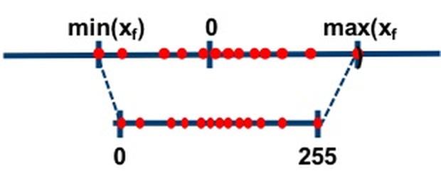 Figure 3. Asymmetric mode, source: https://intellabs.github.io/distiller/algo_quantization.html
Conversely, in symmetric mode, we pick the maximum absolute value between the smallest and largest values of the float range without a zero-point, resulting in both the float range and the quantized range being symmetric around zero.
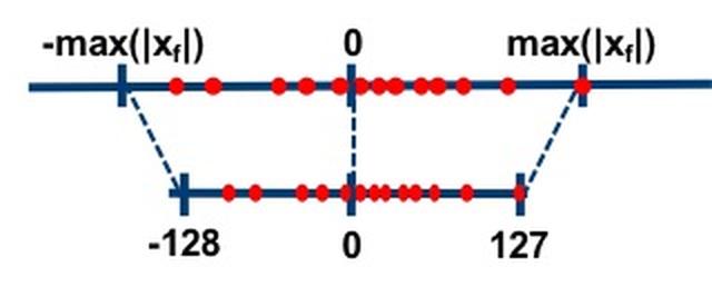 Figure 4. Symmetric mode, source: https://intellabs.github.io/distiller/algo_quantization.html
One of the issues with the approaches presented above, due to the reliance on identifying maximum values, is their sensitivity to outliers which can hugely impact the quantization results.
LLM.int8()
In 2022, Dettmers et al. introduced LLM.int8(), a quantization method addressing the problem of outlier values, frequently present in LLMs’ internal calculations. It uses vector-wise quantization, prioritizing precision for outliers in FP16 format while processing the vast majority of values in INT8 format. With outliers typically making up only around 0.1% of all values, this approach cuts LLM’s memory usage by nearly half (compared to FP16).
LLM.int8() operates in three main stages during matrix multiplication:
- It identifies columns in the input hidden states that contain outlier features using a specific threshold.
- It conducts the matrix multiplication, processing outliers in FP16 and non-outliers in INT8 using vector-wise quantization.
- After dequantizing the non-outlier results from INT8 to FP16, it combines them with the outlier results to produce the complete result in FP16.
Figure 5. Illustration of LLM.int8(), source: https://huggingface.co/blog/hf-bitsandbytes-integration
LLM.int8() was definitely a great development, allowing users to run and experiment with otherwise unavailable models; however, due to its nature (on-the-fly dequantization to FP16 for outlier values), its usage can lead to inference slowdown compared to serving purely 16-bit models.
Our experience with LLM.int8()
The inference slowdown of LLM.int8() mentioned above was confirmed by our experience in a commercial project around LLMs for code completion. According to our experiment results (with 7 billion and 15 billion models from the CodeGen and StarCoder series), the response latency may increase up to 1.5 times. While making it possible to run an inference of StarCoder 15.5B on a single 24GB GPU or two 16GB GPUs (and spend around 4 times less compared to FP16, as shown in Table 1), the speed of code generation was unacceptably low for the model to be usable in the form of a coding assistant. Back then, we had to stick to a smaller model and serve it in FP16. Fortunately, faster quantization algorithms (described below) were proposed not long after.
GPTQ
Introduced by Frantar et al., 2023, the GPTQ (Generative Pre-trained Transformer model Quantization) algorithm is a post-training quantization method, i.e., the weights of an already trained model are converted to lower precision without necessitating any retraining. GPTQ quantizes the model layer by layer, by iteratively going through matrix columns and finding compressed versions of their elements (one for each row) that will yield a minimum mean squared error on a pre-defined calibration dataset. The approach builds and improves on the Optimal Brain Quanization (OBQ) method (Frantar et al., 2022) for solving the layer-wise quantization problem defined above.
GPTQ is currently one of the two most popular quantization techniques (along with AWQ described below). GPTQ-quantized (typically 8-bit and 4-bit) versions of all major newly released LLMs are introduced soon after, and ready-to-use for both further research and commercial applications.
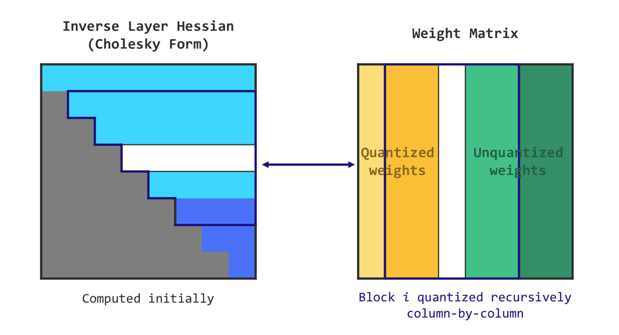 Figure 6. Illustration of GPTQ, source: https://mlabonne.github.io/blog/posts/4_bit_Quantization_with_GPTQ.html
A recently published extension of GPTQ is ExLlamaV2 (EXL2, for short). EXL2, like GPTQ, uses the same optimization method and supports 2, 3, 4, 5, 6 and 8-bit quantization. This format enables you to blend different quantization levels within a model to reach an average bitrate of 2 to 8 bits per weight. Additionally, it makes it possible to apply various quantization levels to each linear layer, resembling sparse quantization, where more crucial weights are quantized with more bits. In this way, it allows Llama2 70B to run on a single 24 GB GPU with a 2048-token context, and 13B models can be used at 2.65 bits within 8 GB of VRAM.
Our experience with GPTQ
Currently, one of the most popular applications of LLMs is retrieval-augmented generation (RAG). In RAG, rather than relying solely on the model’s parameters, the user’s input is first leveraged to extract data from an external source of knowledge, and then both the user query and relevant information are integrated into an LLM prompt, enhancing response generation and mitigating the hallucination issue (to a certain extent). In one of our recent projects concerning RAG in the context of a copilot application for frontline workers, which we developed for a global company from the retail sector, we tested the 4-bit GPTQ version of the powerful open-source model Mixtral 8x7B. With this quantization, we managed to run the model on a single NVIDIA A100 card with 40GB vRAM. For comparison, to run the half-precision model you would need about 90GB GPU vRAM, which exceeds the capacity of the largest available A100 GPU (80GB). As presented in Table 1 (with the example of Llama 2), such memory savings lead to cutting the costs of inference by almost two-thirds. Moreover, as we manually verified the quality of the responses, we observed no difference between the outputs of the quantized model and those of Mixtral served in FP16. In our experiments, 4-bit GPTQ and FP16 models were more or less on par in terms of the speed of text generation.
If you want to learn more about our experience with building RAG systems, consider watching our deeptalk.
AWQ
Another recently popular post-training quantization technique is Activation-aware Weight Quantization, or AWQ (Li et al., 2023), based on the observation that among the LLM’s weights (parameters), not all are equally important for the model’s performance. By identifying a small fraction (0.1%-1%) of so-called salient weights and scaling them up, AWQ effectively reduces their relative quantization error. To pinpoint these salient weight channels, the algorithm analyzes the activation distribution instead of the weight distribution.
Going into more detail, AWQ consists of three main stages:
- profiling activations – run a sample of data through the LLM and record activations, then analyze to identify salient weights.
- optimal scaling – scale up salient weights to minimize quantization error.
- quantization – apply optimal scaling and quantize all weights to INT8/4/2.
The AWQ paper highlights a 3.2-3.3x average speedup compared to Huggingface’s FP16 implementation across various LLMs, but these findings should be treated with caution, as they only report the results for a single, short input prompt. As already stated above, the observed speedup will depend on many factors related to hardware, prompt length and usage patterns. Memory savings, and therefore also cost reduction, in the case of AWQ are similar to those of GPTQ, leading to as much as 3-4 times less money spent on keeping the inference server running.
GGUF
Typically, LLMs are implemented in Python (using its deep learning libraries like PyTorch or Hugging Face transformers), which is not the optimal choice for maximizing inference speed. An interesting project called llama.cpp was started by Georgi Gerganov soon after Meta released their first Llama models in March 2023, with the goal of reimplementing these newly proposed LLMs in C++. Due to its lightweight, portable nature and support for a wide variety of hardware, the project became very popular and matured quickly, currently allowing users to choose from multiple LLMs other than Llama (all implemented in C++).
Apart from implementing the models, the authors of llama.cpp came up with their own quantization algorithm, called k-quants and often referred to as GGUF (after the format in which llama.cpp models are served). This algorithm is less sophisticated than GPTQ or AWQ, but useful in practice, and much superior in terms of inference speed in CPU-only scenarios. There is a wide selection of quantized representations (2-bit, 3-bit, 4-bit, 5-bit, 6-bit and 8-bit), with the possibility to mix different levels of quantization within a single model.
 Figure 7. Phi-2 as an example of a “small language model”, source: https://www.microsoft.com/en-us/research/blog/phi-2-the-surprising-power-of-small-language-models
Our experience with GGUF
We utilized llama.cpp and GGUF-quantized models in our recent PoC project regarding LLMs, or rather SLMs (small language models) deployed on edge devices like mobile phones with Android and only 4 or 6 GB of RAM. We were able to set up the entire RAG pipeline, including the vector index, an embedding model and the generative language model. We found out that 8-bit versions of models like Phi-2 or Gemma were performing reasonably well for retrieval-augmented generation (while for more extreme 4-bit and 5-bit quantizations we saw a significant drop in performance). As of today, running language models on devices with such limited memory is a challenging topic which still needs to be explored further. Nevertheless, there is no doubt that thanks to advancements like GGUF, the recently announced ExecuTorch and various hardware-level optimizations, running a personalized language model on a mobile phone does not seem impossible anymore, with the field of Edge AI continuing to flourish. Deploying language models on edge devices allows one to mitigate the issue with the high cost of hardware and cloud infrastructure required for inference.
Efficient fine-tuning – enabling LLM training on limited hardware
While foundation LLMs of various sizes are already capable of solving many business use cases out-of-the-box (with some time spent on proper prompt engineering, but without the need for any further training), in certain situations there might still be a need to fine-tune them on domain-specific data to reach the satisfactory level of output quality. Compared to the already expensive LLM inference, training a model (either from scratch or fine-tuning an existing one) requires even more powerful hardware, as it is not only the model that needs to fit into memory, but additional space for storing gradients and optimizer states as well. In the case of multi-billion-parameter LLMs, the standard approach to fine-tuning the models by updating all (or some major part) of their parameters is nowadays a procedure only “GPU-rich” companies can afford. The exact calculations are quite complex, with a rule of thumb that the required memory (in gigabytes) is around 12 times the number of model parameters (in billions). An example setup suitable for fine-tuning Llama 2 with 70 billion parameters in the cloud is a cluster of two nodes with 8 A100 GPUs with 80GB VRAM each, resulting in an hourly cost of $61.60 (in the case of GCP). With dozens of hours required to fine-tune an LLM, the total cost of a single model training experiment reaches hundreds or thousands of dollars.
To mitigate this issue, so-called parameter-efficient fine-tuning (PEFT) techniques have been developed, making it possible to effectively tailor pre-trained language models for different downstream tasks, without the requirement to fine-tune every single parameter of the model. Instead, PEFT focuses on fine-tuning only a limited set of additional model parameters, which significantly cuts down on the computational and storage costs linked with fine-tuning LLMs. With parameter-efficient fine-tuning, it is possible to train Llama 2 with 70 billion parameters on a single 80GB GPU, which is 16 times cheaper than with the standard approach.
Quantized inference and parameter-efficient fine-tuning are only selected examples of techniques developed to optimize required memory, decrease response latency, or reduce the time and cost of training LLMs. If you want to know more about the topic, feel free to check out our previous blog post.
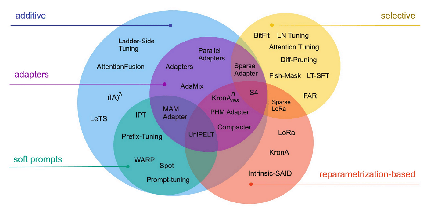 Figure 8. Overview of PEFT techniques, source: https://arxiv.org/pdf/2303.15647.pdf
Various PEFT techniques have been developed and can be divided into categories such as additive, selective, and reparametrization-based methods. Additive methods can be further split into two groups: adapter-like and soft prompt-based methods. In the following sections, we will briefly discuss representative examples of algorithms from these groups. Many of them are implemented as part of the PEFT library, part of the Hugging Face ecosystem, which makes them pretty straightforward to use in practice.
Low-Rank Adaptation (LoRA)
Reparameterization-based methods aim to discover low-dimensional representations of weight matrices. A prominent example of such a method available in PEFT is Low-Rank Adaptation (LoRA, Hu et al., 2021), which is currently the go-to approach for efficient fine-tuning, with new ideas still being built on top of it.
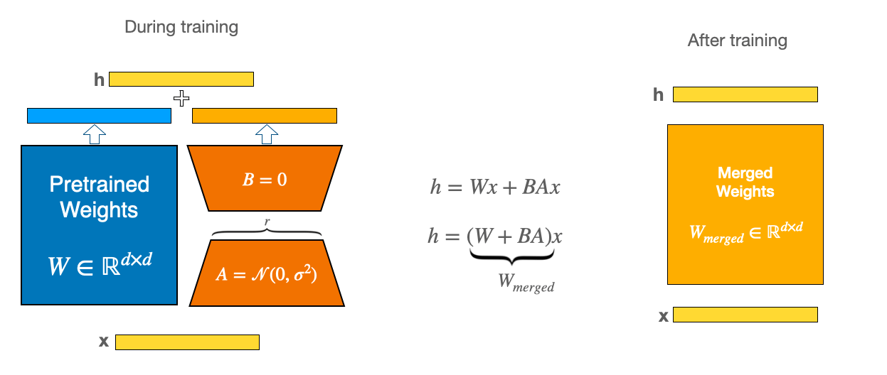 Figure 9. Illustration of LoRA, source: https://huggingface.co/docs/peft/main/en/conceptual_guides/lora
Rather than modifying the parts of the original pre-trained model during fine-tuning, LoRA introduces new weight matrices (marked in orange in the picture above), which are paired with existing parameters (blue); only these newly added weights are then updated during the training process. As LoRA is based on matrix rank decomposition, the new matrices have significantly fewer parameters in total when compared to the original model. The exact numbers vary depending on the rank hyperparameter setting, but the models resulting from LoRA fine-tuning can often be of a quality almost on par with those obtained via full fine-tuning (on much more powerful hardware, hence often even impossible to run), while modifying, e.g., less than 1% of the original parameter count. Moreover, LoRA is an algorithm designed with production environments in mind, as multiple sets of LoRA weights (so-called adapters) can be trained for different use cases, and then easily switched between, while sharing the same underlying pre-trained weights. Additionally, since the original pre-trained weights remain unchanged, the risk of the model forgetting what it had learned before is reduced.
QLoRA
One important extension of the LoRA method available in PEFT is called QLoRA (Dettmers et al., 2023), which is a combination of LoRA and model quantization. It extends LoRA to enhance efficiency by representing the pre-trained weights with low-precision data types, enabling even more extreme reduction of memory required for fine-tuning. In QLoRA, the frozen parameters are stored as FP4 (4-bit floating-point representation newly introduced in the QLoRA paper), but dequantized on demand as training-related calculations and gradient updates are still performed in FP16.
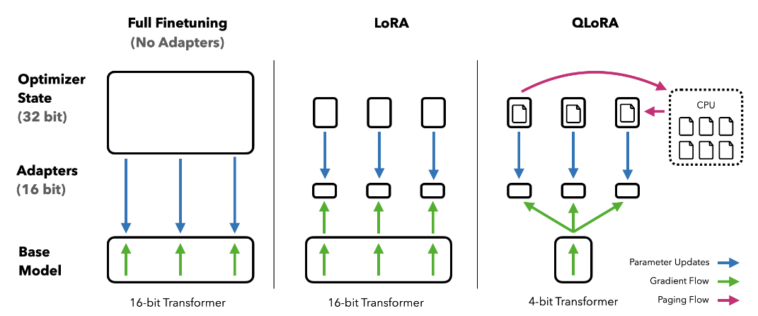 Figure 10. Comparison of full fine-tuning, LoRA and QLoRA, source: https://arxiv.org/pdf/2305.14314.pdf
Our experience with QLoRA
In the abovementioned recent project regarding coding LLMs (language models generating code rather than natural language), our goal was to fine-tune the foundation model to be able to write code in a previously unfamiliar programming language. We only had 48GB of vRAM available at our disposal, but as we leveraged QLoRA, we were able to experiment with fine-tuning both larger models (up to 15 billion parameters with 2048 input tokens) and increasing the context size for smaller models (up to 8192 tokens for a 1-billion-parameter model), with the latter turning out to be the game-changer in the context of coding LLMs. While it was hard to capture the improvement with standard token-level metrics like BLEU or ROUGE, which could only serve as our proxy measurement of quality, the final assessment of the generated code samples conducted by the client (expert in this particular, highly specialized programming language) revealed that the fine-tuned model was superior to the original one. Due to the hardware and budget limitations, we were not able to perform full fine-tuning of analogous models to have a fair comparison, but our experience proves that parameter-efficient fine-tuning techniques, especially when combined with quantization, enable the development of use-case and client-specific LLMs, even with constraints.
Other parameter-efficient fine-tuning methods
Another interesting method found in PEFT is Adaptive Low-Rank Adaptation (AdaLoRA, Zhang et al., 2023). This method builds upon the principles introduced in LoRA but utilizes a distinct form of low-rank matrix decomposition. AdaLoRA optimizes fine-tuning by allocating more trainable parameters to matrices and layers of the model found to be more important.
While LoRA and its variants are currently the most widely used among all the PEFT methods, other noteworthy alternatives exist, as mentioned above.
For example, the goal of additive methods is to enhance a model by introducing a new set of parameters or network layers. During fine-tuning, only these new parameters’ weights are updated. Two such methods are available in PEFT: the Adapters method (Houlsby et al., 2019), which involves introducing small fully-connected networks after the Transformer sub-layers, and the (IA)3 method (Liu et al., 2022), which relies on augmenting the Transformer block with additional parameters.
Another group of methods is based on the concept of prompting. Prompting directs how a language model behaves by changing the input text with a prompt, typically made up of a task description and relevant examples. There are two types of prompts: hard prompts and soft prompts. Hard prompts are manually crafted text prompts using discrete input tokens. Unlike hard prompts, soft prompts cannot be directly viewed and edited in text form. They consist of an embedding, essentially a sequence of numbers, that draws knowledge from the larger model. Soft prompts can be tuned for the input layer only (P-Tuning, Liu et al., 2021 and Prompt Tuning, Lester et al., 2021) or for all layers (Prefix Tuning, Li and Liang, 2021).
Summary
In this article, we discussed the recent trend in the field of generative AI – the democratization of LLMs, which is about making these text-processing models accessible to everyone by reducing the hardware (and the associated cost) requirements. Recent advances such as new model quantization and parameter-efficient fine-tuning techniques not only make it possible to run or fine-tune one’s own LLM on their personal computer or edge device for fun or small-scale projects. Much more importantly, this also means that LLMs are becoming cheaper for businesses who want to incorporate AI into their existing products or processes, or unlock completely new ideas and functionalities previously impossible to implement.
At deepsense.ai, we have hands-on experience with applying the methods described above in commercial projects such as the development of a coding assistant for a highly specialized programming language, or an LLM-powered mobile application for field workers in the retail sector. Our experiments confirm the effectiveness and importance of these methods in turning the recent advancements in generative AI into business value.
If the article has got you interested in potential use cases of LLMs at your company, we invite you to explore our LLM Discovery Workshops offering, where you can learn more from our experts and find out how your business can benefit from cutting-edge technology.
The post Reducing the cost of LLMs with quantization and efficient fine-tuning: how can businesses benefit from Generative AI with limited hardware? appeared first on deepsense.ai.
